Asynchronous counter / Ripple counter – Circuit and timing diagram

An asynchronous counter, also known as a ripple counter, is a type of digital counter used in digital electronics to count clock pulses.

It is constructed using a series of flip-flops connected so that only the first flip-flop receives the external clock signal, while the clock input of each subsequent flip-flop is driven by the output of the preceding flip-flop.

As a result, the change in state propagates from one flip-flop to the next, creating a ripple effect.

Asynchronous counters operate without a common clock signal for all flip-flops. Unlike synchronous counters, in which all flip-flops receive the same external clock, the flip-flops in an asynchronous counter change state sequentially.

An asynchronous counter can be designed as an up counter, down counter, or up/down counter, depending on the required counting sequence and control inputs.

Asynchronous counters are commonly used in digital circuits for frequency division, event counting, and simple counting applications where the propagation delay is acceptable.

However, because the flip-flops change state one after another, their propagation delays accumulate as the count propagates through the circuit.

Therefore, asynchronous counters are generally slower than synchronous counters and are less suitable for high-speed counting applications.

In this article, we will explore the working principle, circuit design, and timing diagrams of asynchronous counters, including asynchronous up counters, down counters, and up/down counters.

We will also examine how the clock signal propagates through the flip-flops and produces the ripple effect in a digital counter. Also, learn the design of ripple/synchronous counter.

For the design of the asynchronous counter, T flip-flops are used. Because the output toggles in T flip-flop. In other words, this flip-flop produces complementing output. That is, if 0 is given as the input, 1 is produced at the output and vice versa.

The flip-flop used for the asynchronous counter is negative edge-triggered flip-flops. It means, the flip-flop will change its state at the falling edge of the clock pulse.

2-bit asynchronous up counter

For a 2-bit asynchronous counter, 2 flip-flops are used as shown in the below figure. It is an up counter, where the count is incremented for each clock pulse. A 2-bit counter will have 2² = 4 distinct states(00, 01, 10, 11).

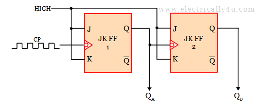
The clock pulse input is given to the first flip-flop only. The output(Q_A) of the first flip-flop is fed as the clock input for the second flip-flop. The HIGH or logic 1 is maintained at the T-input of both flip-flops.

The clock pulse is digitally counted at the output Q_A and Q_B, where Q_A is the Least significant bit(LSB) and Q_B is the most significant bit(MSB).

Operation

Let us assume the initial state of flip-flop as Q_BQ_A = 00. During the first clock pulse, that is at the falling edge of the clock pulse, JK FF1 will toggle its output state to logic 1. For the next clock pulse, again JK FF1 will toggle its output to logic 0. The toggling of JK FF1 continues for each clock pulse.

Now, What about the state of JK FF2 ?

The output of the first flip-flop(JK FF1) is given as a clock pulse input for the second flip-flop(JK FF2). Whenever the Q_A output goes high, at the falling edge of its output, the JK FF2 will get triggered. When the JK FF2 gets triggered, it produces a toggled output.

As we have assumed the initial state of JK FF2 as Q_B = 0, the output will get toggled to Q_B = 1. This output again toggles, when the output of JK FF1 goes high HIGH.

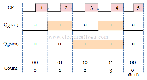
The change of state of flip-flops for each occurrence of the clock pulse is shown in the below timing diagram. As you can observe from the timing diagram, the counter counts from o0 to 11. After reaching 11, the counter resets to 00 and starts to count from 00 again.

3-bit asynchronous up counter

The 3-bit asynchronous or ripple up counter is similar to the 2-bit ripple up counter. Here for a 3-bit counter, an additional flip-flop is added. Thus for the 3-bit asynchronous counter, 3 T-flip-flops are used.

This counter consists of 2³ = 8 count states(000, 001, 010, 011, 100, 101, 110, 111). The counter counts the incoming pulses starting from 0 to 7.

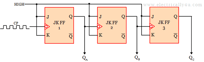
The above circuit shows the circuit diagram of a 3-bit asynchronous up counter, in which the clock pulse is given as clock input for JK FF1. For the other flip-flops, the clock input is fed from the output of previous flip-flops.

The clock pulse count is noted at the output of each flip-flop(Q_CQ_BQ_A), where Q_A is the LSB and Q_C is the MSB.

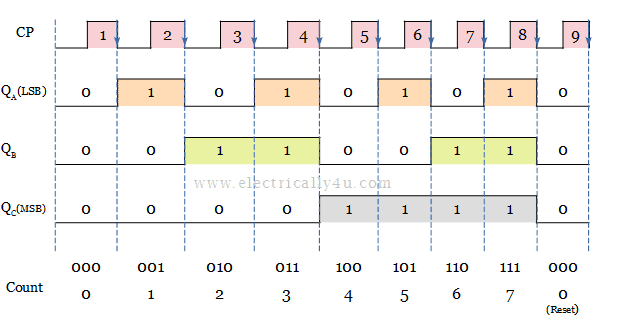
The operation is the same as the 2-bit asynchronous up counter. At the falling edge of each clock pulse, the output of JF FF1 toggles. For each logic HIGH output(Q_A = 1) of JK FF1, at its falling edge, JK FF2 will toggle the output(Q_B). Similarly, for each logic HIGH output(Q_B = 1) of JK FF2, JK FF3 will toggle the output(Q_C).

The below figure shows the timing diagram of the 3-bit ripple counter, which shows the change of state of each flip-flop during each clock pulse. In this type, the counter resets to 000, after counting up to 111.

3-bit asynchronous down counter

The down counter will count the clock pulses from maximum value to zero. In other words, for each clock pulse, the count value is decremented.

The below diagram shows the 3-bit asynchronous down counter. Since it is a 3-bit counter, 3 negative edge-triggered flip-flops are used. The clock pulse input is given only to the first flip-flop. The clock input of the remaining flip-flops is triggered by the Q output of the previous flip-flop.

Since it is down counter, the 3-bit count value is measured from the (Q_C‘Q_B‘Q_A‘), where Q_C‘ is the MSB and Q_A‘ is the LSB.

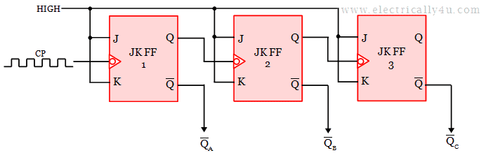
The operation is the same as that of the 3-bit asynchronous up counter. If the output is taken at the normal Q output of each flip flop, then it is an up counter. If the output is taken at the complemented output (Q’) of each flip flop, it is said to be the down counter.

The change of state of each flip flop with respect to the clock pulse and the count value is shown in the below timing diagram.

In this diagram, the output waveform Q_C, Q_B, Q_A represents the normal Q output of JK FF3, JK FF2 and JK FF1 respectively. In the below waveform, Q_C‘, Q_B‘, Q_A‘ represents the complemented output from of JK FF3, JK FF2 and JK FF1 respectively.

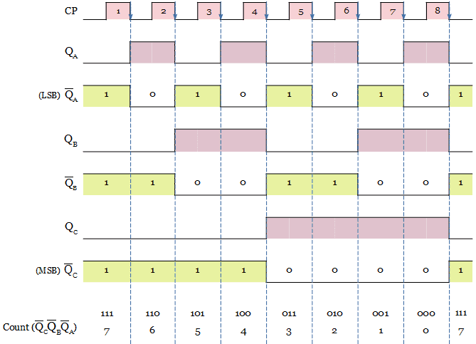
The count value can be observed from the complemented outputs. The counter value starts from 111 and decrements its value for each clock pulse. After reaching 000, the counter resets to the maximum value(111) and starts to decrement again for the next clock pulse.

Asynchronous Up/Down counter (or) Bidirectional counter

For asynchronous up/down counter, control input is necessary for the control of the operation as up or down counter.

When the control input is 0, in the following figure, the AND gates 1 and 3 are disabled. It enables gate 2 and 4, which means, Q’ output of first and second flip-flop drives the clock input of JK FF2 and JK FF3 respectively. In this case, the counter will perform the operation of the down counter.

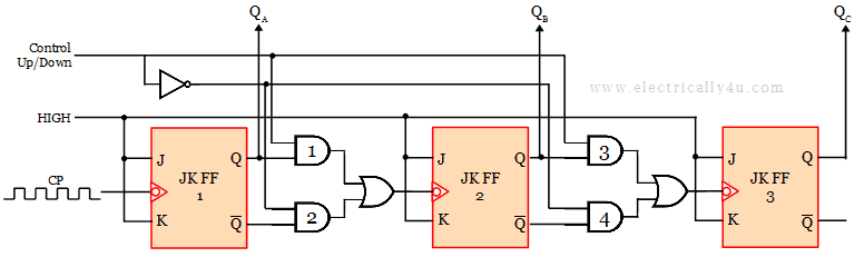
When the control input is 1, gates 1 and 3 are enabled and gates 2 and 4 are disabled. This makes a way for the Q output of flip-flops to drive the clock input of the next stage flip-flop. Now, the counter will perform the up counter operation.

What is Binary Ripple Counter?

A binary ripple counter is a type of asynchronous counter constructed using a series of flip-flops, typically JK flip-flops, connected in cascade. It is also known as an n bit ripple counter, where “n” represents the number of flip-flops used. It is similar to asynchronous up counter.

Each flip-flop operates in toggle mode, toggling its state on the falling edge (negative edge) of the clock signal it receives. The output frequency of each flip-flop is half that of its input clock frequency, resulting in a frequency division by 2 for each stage.

Consequently, the output frequency of the most significant flip-flop (MSB) is the input clock frequency divided by 2ⁿ.

The binary ripple counter counts in binary number sequence from 0 up to 2^n-1 (for example, a 3 bit ripple counter counts from 000 to 111).

Because the flip-flops are not clocked simultaneously and the state changes propagate sequentially, the binary ripple counter exhibits propagation delay.

This delay accumulates through all the flip-flops, limiting the maximum clock frequency at which the counter can operate reliably.

Applications of Asynchronous Counter

Asynchronous counters, also known as ripple counters, are widely used in digital electronics due to their simple design and effectiveness in various counting and timing applications. Some key applications include:

1. Frequency Division: Asynchronous counters are commonly used to divide the frequency of clock signals. Each flip-flop divides the input frequency by two, making ripple counters ideal for creating frequency dividers in digital circuits.
2. Event Counting: They are used in event counters where the count of occurrences of an event is required. For example, counting pulses in digital meters or measuring the number of items passing a sensor.
3. Digital Clocks: Asynchronous counters are employed in digital clocks to count seconds, minutes, and hours by cascading multiple counters.
4. Multiplexing: They find applications in multiplexing circuits where sequential selection of input lines is needed.
5. Simple Binary Counters: Due to their straightforward design using only one flip flop clocked externally and the next flip flop triggered by the output of the previous, asynchronous counters are suitable for simple binary counting tasks.
6. Mod-n Counters: By using combinational logic with asynchronous counters, specific count sequences can be generated, such as mod 8 counters or mod 16 counters, useful in various timing and control circuits.
7. Pulse Generation: They can be used to generate specific timing pulses or bit patterns required in digital systems.
8. Digital Frequency Meters: Asynchronous counters serve as the counting element in frequency measurement devices.

While asynchronous counters are slower compared to synchronous counters due to ripple delays, their simplicity and ease of implementation make them valuable in applications where high-speed operation is not critical.