
Nodal Analysis
Key Takeaways
- Nodal analysis uses Kirchhoff’s Current Law (KCL) and Ohm’s Law to solve unknown node voltages in an electrical circuit; every branch current and power can then be derived from those voltages.
- Choosing a reference node (marked with a ground symbol and set to 0 V) reduces the number of unknowns to N − 1, where N is the total number of nodes.
- The resulting nodal equations can be arranged into a compact matrix equation GV = I and solved by Gaussian elimination, matrix inversion, or software for large circuits.
- The nodal analysis method extends directly to AC circuits (using complex impedance and phasors), dependent sources, and nonlinear circuits through modified nodal analysis (MNA).
- Nodal analysis is complementary to mesh analysis; it tends to produce fewer equations in circuits with many current sources or non-planar topologies.
Introduction to Nodal Analysis
Nodal analysis is one of the most widely taught and used techniques for analyzing electrical circuits. It is a fundamental topic in undergraduate circuit analysis courses and is also used in circuit simulation tools such as SPICE.
Engineers often use nodal analysis for quickly determining unknown voltages and currents in electrical circuits.
The main goal of nodal analysis is to determine the voltage at each circuit node with respect to a reference node, usually called the ground node.
Once the node voltages are known, the branch currents, voltage drops, and power associated with the circuit elements can be calculated using basic circuit relationships.
In this article, Elpedia presents nodal analysis as a systematic and repeatable method based on Kirchhoff’s Current Law (KCL) and fundamental circuit principles.
The method can be applied to simple circuits containing a few components as well as complex circuits containing many interconnected elements.
This article explains the basic procedure for nodal analysis, including reference nodes, node-voltage equations, supernodes, and matrix-based solutions. It also introduces nodal analysis for AC circuits and compares it with mesh analysis.
By the end of the article, you will have a clear understanding of how to apply nodal analysis to a wide range of electrical circuits.
Fundamental Laws Behind Nodal Analysis
Three fundamental principles are closely associated with nodal analysis: Kirchhoff’s Current Law (KCL), Ohm’s Law, and Kirchhoff’s Voltage Law (KVL).
Kirchhoff’s Current Law (KCL), which is the primary engine, states that the algebraic sum of currents at a node is zero. It is based on the principle of conservation of electric charge: charge cannot accumulate indefinitely at an ideal circuit node. Therefore, the total current entering a node must equal the total current leaving it.
For a node with three branch currents, KCL can be written as:
![\[i_1 + i_2 +i_3 = 0\]](https://elpedia.com/wp-content/ql-cache/quicklatex.com-cf8084ea4e05680e3fb010a938f2d2b2_l3.png "Rendered by QuickLaTeX.com")
The signs depend on the chosen current convention. For example, currents leaving the node may be considered positive and currents entering the node negative. Either convention is valid as long as it is applied consistently.
Ohm’s Law relates voltage, current, and resistance in a resistive element. For a resistor connected between two nodes with voltages and , the current through the resistor can be written as:
![\[i = \frac{V_1 - V_2}{R} \]](https://elpedia.com/wp-content/ql-cache/quicklatex.com-d5c8cb074a30c8f52244adcf585112b8_l3.png "Rendered by QuickLaTeX.com")
This relationship is particularly important in nodal analysis because it allows each branch current to be expressed in terms of the known or unknown node voltages.
For sinusoidal steady-state AC circuits, resistance can be generalized to complex impedance. The corresponding branch-current relationship is:
![\[i = \frac{V_1 - V_2}{Z} \]](https://elpedia.com/wp-content/ql-cache/quicklatex.com-74b0ece53b3096b44b0e556f5db0a46a_l3.png "Rendered by QuickLaTeX.com")
For an ideal inductor and capacitor, their impedances are:
![\[Z_L = j\omega L \]](https://elpedia.com/wp-content/ql-cache/quicklatex.com-d9ca88631eecfc915c43b81efacc08d7_l3.png "Rendered by QuickLaTeX.com")
![\[Z_C = \frac{1}{j\omega C} \]](https://elpedia.com/wp-content/ql-cache/quicklatex.com-1036603e4f7ca8008f572c80a09fa8f6_l3.png "Rendered by QuickLaTeX.com")
where is the imaginary unit and is the angular frequency.
Kirchhoff’s Voltage Law (KVL) states that the algebraic sum of voltages around any closed loop is zero. Unlike mesh analysis, nodal analysis does not normally require a separate KVL equation for each loop.
Instead, branch currents are determined from node voltages using the appropriate element relationships, while KCL is applied at the nodes.
Thus, KCL provides the governing equations for nodal analysis, while the element voltage-current relationships allow those equations to be written in terms of node voltages.
KVL remains a fundamental law of circuit theory and is consistent with the resulting circuit solution.
Basic Terminology: Nodes, Nodal Voltage, and Reference Node
Before applying nodal analysis, it is important to understand three basic concepts: node, nodal voltage, and reference node.
A node is a point in an electrical circuit where two or more circuit elements are connected. All points connected by an ideal wire, which has zero resistance, are considered to be at the same electrical potential and therefore belong to the same node, regardless of how far apart they appear in a circuit diagram.
An essential node is a node at which three or more circuit elements or branches meet. These nodes are particularly important in nodal analysis because applying Kirchhoff’s Current Law (KCL) at them provides useful equations for determining the unknown node voltages.
A nodal voltage, or node voltage, is the electric potential of a node measured with respect to a selected reference node. Since voltage is a potential difference, a node voltage is always defined relative to the reference node.
For example, if node A has a voltage VA with respect to the reference node, then:
![\[V_A = V_{\text{A}} - V_{\text{reference}}\]](https://elpedia.com/wp-content/ql-cache/quicklatex.com-16cf115581b5b635786facfafc0b0114_l3.png "Rendered by QuickLaTeX.com")
If the reference node is assigned 0 V, then the numerical value of VA is simply the potential of node A relative to that reference.
It is important to distinguish node voltage from the voltage between any two arbitrary nodes. The voltage between nodes A and B is:
![\[V_{AB}=V_A-V_B\]](https://elpedia.com/wp-content/ql-cache/quicklatex.com-2e751e6fa5f42a04d75dd3bf6a0a3183_l3.png "Rendered by QuickLaTeX.com")
Thus, once the node voltages are known, the voltage between any two nodes can be determined by subtracting their respective node voltages.
The reference node is the node chosen as the common reference point for measuring all other node voltages. It is usually assigned a voltage of 0 V and is commonly represented by a ground symbol in the circuit diagram.
The reference node does not necessarily have to be physically connected to earth or ground. In circuit analysis, the ground symbol usually indicates that the node has been selected as the 0 V reference.
The reference node can be chosen freely, but selecting a node connected to several circuit elements can often simplify the nodal equations. In many circuits, a node connected to the negative terminal of a voltage source or to several branches is a convenient choice.
If a circuit contains N distinct nodes, one node is selected as the reference node. Its voltage is already known as 0 V, so only the remaining N-1 node voltages need to be determined.
Therefore:
![\[\boxed{\text{Number of unknown node voltages}=N-1}\]](https://elpedia.com/wp-content/ql-cache/quicklatex.com-5603e4e6e85a18b0c266fdea5c86bd6f_l3.png "Rendered by QuickLaTeX.com")
This is one of the basic counting rules used in nodal analysis.
Nodal analysis is a systematic circuit-analysis technique based primarily on Kirchhoff’s Current Law (KCL). By applying KCL at the appropriate nodes and expressing branch currents in terms of node voltages, the unknown node voltages can be determined.
Once these voltages are known, branch currents, voltage differences, and power can also be calculated.
Nodal analysis is closely related to mesh analysis, but the two methods use different primary variables. Nodal analysis uses node voltages as the unknown variables, whereas mesh analysis uses mesh currents.
Steps to solve nodal analysis method
- The nodal analysis makes the analysis simpler only if the circuit has only current sources. If any voltage source is present in the circuit, prior to the nodal analysis, the voltage source has to be converted into the current source by the source transformation method.
Let us consider a simple circuit, as shown below
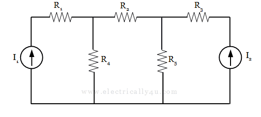
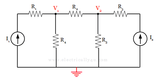
- Identify all the principal nodes in the circuit and choose a reference node. All the nodes except the reference node are numbered and the corresponding voltages are designated as V1, V2,… The reference node can be grounded.
In the considered circuit, there are two principal nodes and are designated as V1 and V2. The bottom node is considered a reference node and is grounded for identification.
- Assign the currents to each branch. Express the branch currents in terms of node voltages by using Ohm’s Law.
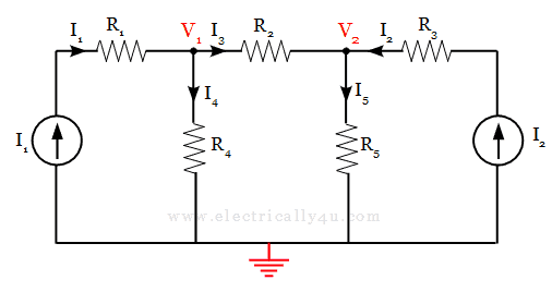
The branch currents can be expressed as
![\[ I_3 = \frac{V_1 - V_2}{R_2}, I_4 = \frac{V_1 - 0}{R_4}, I_5 = \frac{I_5 - 0}{R_5} \]](https://elpedia.com/wp-content/ql-cache/quicklatex.com-920b1d470b5477bb687c35333b868e4c_l3.png "Rendered by QuickLaTeX.com")
- Apply Kirchoff’s Current Law(KCL) for all the nodes(except reference node) and write the nodal equations.
- Solve the KCL equations to get the node voltages.
Working with Supernodes and Floating Voltage Sources
A supernode is formed when an ideal voltage source connects two non-reference nodes in a circuit. Since the voltage source establishes a fixed potential difference between these nodes, the current through the voltage source cannot be directly expressed using Ohm’s law.
Therefore, writing separate KCL equations at the two nodes without considering the voltage constraint is not sufficient. Instead, both nodes and the voltage source connecting them are treated as a single analytical unit called a supernode.
The procedure for applying nodal analysis with supernodes:
- Identify the supernode: Draw a boundary around the two non-reference nodes connected by the voltage source, including the voltage source itself.
- Apply Kirchhoff’s Current Law (KCL): Write one KCL equation for the supernode as a whole by considering the currents flowing between the supernode and the external circuit. The current through the internal voltage source is not included because it remains inside the supernode boundary.
- Write the voltage constraint equation: Express the voltage relationship between the two nodes according to the source polarity. For a voltage source with its positive terminal connected to node 1 and its negative terminal connected to node 2, V1 – V2 = Vs. If the source polarity is reversed, the equation becomes V2 – V1 = Vs.
- Solve the equations: Combine the supernode KCL equation, the voltage constraint equation, and any other required nodal equations to determine the unknown node voltages.
Supernodes simplify nodal analysis by eliminating the need to determine the current through an ideal voltage source directly. The voltage constraint equation provides the additional relationship needed to determine the node voltages.
Whenever an ideal voltage source connects two non-reference nodes, a supernode can be used to formulate the nodal equations. If a voltage source connects a node directly to the reference node, the voltage at that node is already known, so a supernode is generally unnecessary.
In matrix-based nodal analysis, the voltage constraint equations must be incorporated along with the KCL equations.
For a supernode containing two non-reference nodes, one combined KCL equation and one voltage constraint equation can be used in place of the two individual KCL equations.
This preserves the required number of independent equations for determining the unknown node voltages.
Solved Problem 1
Determine the current through each resistor in the given circuit using nodal analysis.
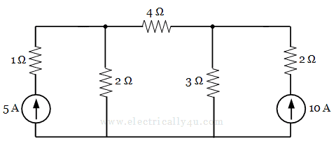
In this circuit, there are two nodes, which are designated as V1 and V2. The bottom nodes are together considered as a reference node(grounded). The currents are assigned in each branch and the circuit is redrawn as below.
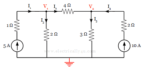
Apply Kirchoff’s Current Law at node 1,
![\[ I_1 = I_2 + I_3 \]](https://elpedia.com/wp-content/ql-cache/quicklatex.com-9c0fbb85977e0b57dfa67aec6021e872_l3.png "Rendered by QuickLaTeX.com")
![\[ 5 = \frac{V_1 - V_2}{4} + \frac{V_1}{2} \]](https://elpedia.com/wp-content/ql-cache/quicklatex.com-f900eb8361363a5e803788c2f775b2f3_l3.png "Rendered by QuickLaTeX.com")
![\[0.25 V_1 - 0.25V_2 + 0.5V_1 = 5\]](https://elpedia.com/wp-content/ql-cache/quicklatex.com-fcd1818c66ea54c43e6127a6ce663985_l3.png "Rendered by QuickLaTeX.com")
![\[ 0.75V_1 - 0.25V_2 = 5 --->(1)\]](https://elpedia.com/wp-content/ql-cache/quicklatex.com-5c2d9d6ba24d59dc9613b08e373d1522_l3.png "Rendered by QuickLaTeX.com")
Apply KCL at node 2,
![\[I_4 + I_2 = I_5 \]](https://elpedia.com/wp-content/ql-cache/quicklatex.com-59ab447988a66befc1492fe021cabcf6_l3.png "Rendered by QuickLaTeX.com")
![\[10 + \frac{V_1 - V_2}{4} = \frac{V_2}{3} \]](https://elpedia.com/wp-content/ql-cache/quicklatex.com-5098a627d71f66469c51f59ddeb24e23_l3.png "Rendered by QuickLaTeX.com")
![\[ 0.25V_1 - 0.25V_2 - 0.33V_2 = -10 \]](https://elpedia.com/wp-content/ql-cache/quicklatex.com-e06b670ad24aa59ca839c13be9936285_l3.png "Rendered by QuickLaTeX.com")
![\[ 0.25V_1 - 0.58V_2 = -10 --->(2)\]](https://elpedia.com/wp-content/ql-cache/quicklatex.com-9a747c1ecf92ba8e07b84b3da75f7396_l3.png "Rendered by QuickLaTeX.com")
The above two equations are written in matrix form, as shown below,
![\[ \begin{bmatrix} 0.75 & -0.25 \\ 0.25 & -0.58 \end{bmatrix} \begin{bmatrix} V_1 \\ V_2 \end{bmatrix} = \begin{bmatrix} 5 \\ -10 \end{bmatrix} \]](https://elpedia.com/wp-content/ql-cache/quicklatex.com-be25df2745c0a55e6290b612a392f379_l3.png "Rendered by QuickLaTeX.com")
Applying Cramer’s rule, we get
![\[ \Delta = \begin{vmatrix} 0.75 & -0.25 \\ 0.25 & -0.58 \end{vmatrix} = -0.435 + 0.0625 = -0.373 \]](https://elpedia.com/wp-content/ql-cache/quicklatex.com-dd2acadecfee27a69da56ffbc177c44c_l3.png "Rendered by QuickLaTeX.com")
![\[ \Delta_1 = \begin{vmatrix} 5 & -0.25 \\ -10 & -0.58 \end{vmatrix} = -2.9 - 2.5 = -5.4 \]](https://elpedia.com/wp-content/ql-cache/quicklatex.com-08c5610324724a2adbfd00a22807964e_l3.png "Rendered by QuickLaTeX.com")
![\[ \Delta_2 = \begin{vmatrix} 0.75 & 5 \\ 0.25 & -10 \end{vmatrix} = -7.5 - 1.25 = -8.75 \]](https://elpedia.com/wp-content/ql-cache/quicklatex.com-761c7c5e232869956e9b1ecd2b139085_l3.png "Rendered by QuickLaTeX.com")
Now, the node voltages is determined
![\[V_1 = \frac{\Delta_1}{\Delta} = \frac{-5.4}{-0.373} = 14.47 V\]](https://elpedia.com/wp-content/ql-cache/quicklatex.com-1d218cec29423b4dcf3d4192b2589049_l3.png "Rendered by QuickLaTeX.com")
![\[V_2 = \frac{\Delta_2}{\Delta} = \frac{-8.75}{-0.373} = 23.46 V\]](https://elpedia.com/wp-content/ql-cache/quicklatex.com-9e109138845520d2447ba5c6d25f286f_l3.png "Rendered by QuickLaTeX.com")
The branch currents are determined as follows
![\[I_1 = 5 A\]](https://elpedia.com/wp-content/ql-cache/quicklatex.com-41c435db0c1e5301c6374216fa98ca56_l3.png "Rendered by QuickLaTeX.com")
![\[I_2 = \frac{V_1 - V_2}{4} = \frac{14.47 - 23.46}{4} = -2.24 A \]](https://elpedia.com/wp-content/ql-cache/quicklatex.com-19eafb7d99e8831c25921a37bde6ed44_l3.png "Rendered by QuickLaTeX.com")
![\[I_3 = \frac{V_1}{2} = \frac{14.47}{2} = 7.23 A\]](https://elpedia.com/wp-content/ql-cache/quicklatex.com-0e54dcaaa9fe479762cbb2f26c909c44_l3.png "Rendered by QuickLaTeX.com")
![\[ I_4 = 10 A\]](https://elpedia.com/wp-content/ql-cache/quicklatex.com-e2acc05f411c9673cca66846bf2a55f4_l3.png "Rendered by QuickLaTeX.com")
![\[ I_5 = \frac{V_2}{3} = \frac{23.46}{3} = 7.82 A \]](https://elpedia.com/wp-content/ql-cache/quicklatex.com-9ea8ab6babc01e498d2615241693fe81_l3.png "Rendered by QuickLaTeX.com")
Solved Problem 2
Find the different nodal voltages in the given circuit.
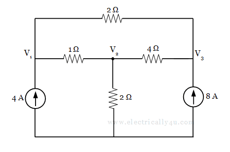
In this circuit, there are three given nodes, which are designated as V1, V2 and V3. For these three nodes, we have to write the current equations by applying KCL. Before that, let us assign the current in each branches and redraw the circuit.
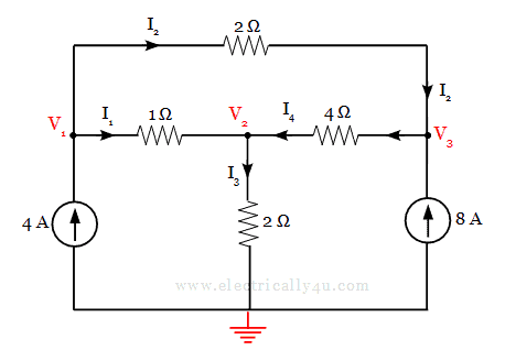
Apply Kirchoff’s Current Law at node 1,
![\[4 = I_1 + I_2\]](https://elpedia.com/wp-content/ql-cache/quicklatex.com-bfa8d08adb1317180116b847c4e350aa_l3.png "Rendered by QuickLaTeX.com")
![\[ 4 = \frac{V_1 - V_2}{1} + \frac{V_1 - V_3}{2}\]](https://elpedia.com/wp-content/ql-cache/quicklatex.com-26df22eec4170c71a83d8026e8df7a37_l3.png "Rendered by QuickLaTeX.com")
![\[1.5V_1 - V_2 - 0.5V_3 = 4 --->(1) \]](https://elpedia.com/wp-content/ql-cache/quicklatex.com-224a07d0e4ed0da1fd5f3e19fc859ddc_l3.png "Rendered by QuickLaTeX.com")
Apply KCL at node 2,
![\[I_1 + I_4 = I_3\]](https://elpedia.com/wp-content/ql-cache/quicklatex.com-069001ae25fea74921aebc9355cd855c_l3.png "Rendered by QuickLaTeX.com")
![\[\frac{V_1 - V_2}{1} + \frac{V_3 - V_2}{4} = \frac{V_2}{2}\]](https://elpedia.com/wp-content/ql-cache/quicklatex.com-690a3f2418f5c203217e81c22fb135de_l3.png "Rendered by QuickLaTeX.com")
![\[V_1 - 1.25V_2 - 0.25V_3 = 0 --->(2)\]](https://elpedia.com/wp-content/ql-cache/quicklatex.com-889dcd2f978264ca7745bfabd78acb4a_l3.png "Rendered by QuickLaTeX.com")
Apply KCL at node 3,
![\[8 + I_2 = I_4\]](https://elpedia.com/wp-content/ql-cache/quicklatex.com-3c69958e94905d52703e97d82a67189a_l3.png "Rendered by QuickLaTeX.com")
![\[8 + \frac{V_1 - V_3}{2} = \frac{V_3 - V_2}{4}\]](https://elpedia.com/wp-content/ql-cache/quicklatex.com-97bf7f55d675eb12f7172fbe2675a815_l3.png "Rendered by QuickLaTeX.com")
![\[0.5V_1 + 0.25V_2 - 0.75V_3 = -8 --->(3)\]](https://elpedia.com/wp-content/ql-cache/quicklatex.com-ef79ac2a74916ec4d105852a13ad62de_l3.png "Rendered by QuickLaTeX.com")
The above three equations are written in matrix form, as shown below,
![\[ \begin{bmatrix} 1.5 & -1 & -0.5 \\ 1 & -1.25 & -0.25 \\ 0.5 & 0.25 & -0.75 \end{bmatrix} \begin{bmatrix} V_1 \\ V_2 \\ V_3 \end{bmatrix} = \begin{bmatrix} 4 \\ 0 \\ -8 \end{bmatrix} \]](https://elpedia.com/wp-content/ql-cache/quicklatex.com-7a89f05f6fbdd49ca78836729ab46cf2_l3.png "Rendered by QuickLaTeX.com")
Applying Cramer’s rule, we get
![\[ \Delta = \begin{vmatrix} 1.5 & -1 & -0.5 \\ 1 & -1.25 & -0.25 \\ 0.5 & 0.25 & -0.75 \end{vmatrix}\]](https://elpedia.com/wp-content/ql-cache/quicklatex.com-27b4ecaa959c600a342b862e8f60e70b_l3.png "Rendered by QuickLaTeX.com")
![\[\Delta = 1.5(0.94+0.063)+1(-0.75+0.125)-0.5(0.25+0.625) = 0.442 \]](https://elpedia.com/wp-content/ql-cache/quicklatex.com-28c65034276221bb386e58277afc981d_l3.png "Rendered by QuickLaTeX.com")
![\[ \Delta_1 = \begin{vmatrix} 4 & -1 & -0.5 \\ 0 & -1.25 & -0.25 \\ -8 & 0.25 & -0.75 \end{vmatrix} = 4(0.94+0.063)+1(0-2)-0.5(0-10)=7.012 \]](https://elpedia.com/wp-content/ql-cache/quicklatex.com-240b5b1a56a4278219dfacbaae16eb59_l3.png "Rendered by QuickLaTeX.com")
![\[ \Delta_2 = \begin{vmatrix} 1.5 & 4 & -0.5 \\ 1 & 0 & -0.25 \\ 0.5 & -8 & -0.75 \end{vmatrix} = 1.5(0-2)-4(-0.75+0.125)-0.5(-8+0)=3.5 \]](https://elpedia.com/wp-content/ql-cache/quicklatex.com-485fd848a647063017fe0db5a92914eb_l3.png "Rendered by QuickLaTeX.com")
![\[ \Delta_3 = \begin{vmatrix} 1.5 & -1 & 4 \\ 1 & -1.25 & 0 \\ 0.5 & 0.25 & -8 \end{vmatrix} = 1.5(10-0)+1(-8-0)+4(0.25+0.625)=10.5 \]](https://elpedia.com/wp-content/ql-cache/quicklatex.com-492edb38bba88c20b583c3a8c09a859a_l3.png "Rendered by QuickLaTeX.com")
Now, the node voltages are determined
![\[V_1 = \frac{\Delta_1}{\Delta} = \frac{7.012}{0.442} = 15.86 V\]](https://elpedia.com/wp-content/ql-cache/quicklatex.com-fae41bb9ec3b3d0b2f1449fbb3142a1a_l3.png "Rendered by QuickLaTeX.com")
![\[V_2 = \frac{\Delta_2}{\Delta} = \frac{3.5}{0.442} = 7.92 V\]](https://elpedia.com/wp-content/ql-cache/quicklatex.com-171d3b18f7f71873fe98315d4dba5621_l3.png "Rendered by QuickLaTeX.com")
![\[V_3 = \frac{\Delta_3}{\Delta} = \frac{10.5}{0.442} = 23.76 V\]](https://elpedia.com/wp-content/ql-cache/quicklatex.com-0c210a2852316cdee1a472b9d002ccc5_l3.png "Rendered by QuickLaTeX.com")
Nodal Analysis for AC Circuits
Nodal analysis can handle both DC and AC circuits. In sinusoidal steady-state AC analysis, nodal voltages become complex phasors, and resistances are replaced by complex impedance values:
The same KCL-based procedure applies. Write nodal equations in terms of complex nodal voltages and impedances, then assemble them into a complex matrix equation YV = I, where Y is the admittance matrix with complex entries.
Comparison of Nodal Analysis and Mesh Analysis
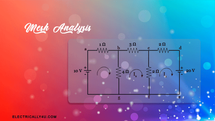
Mesh analysis is a KVL-based technique that solves for loop currents instead of node voltages. It works only in planar circuits (circuits that can be drawn flat without crossing wires).
Factor | Nodal analysis | Mesh analysis |
|---|---|---|
Core law | KCL | KVL |
Unknowns | Node voltages (N−1) | Loop currents |
Works for non-planar circuits | Yes | No |
Preferred when | Many current sources, high node count | Many voltage sources, few loops |
Typical equation count (textbook circuits) | Often ~1/3 fewer than mesh | Varies |
Nodal analysis often results in fewer equations compared to mesh analysis for circuits with fewer nodes than loops. For solving circuits where node voltages are the desired output (power distribution, signal integrity), nodal analysis is the natural choice.
Mesh analysis may be simpler for series-dominant circuits with several voltage sources. Both methods rely on the same fundamental laws; the choice depends on circuit structure and which quantities you need.
Engineers working on hand calculations sometimes use a hybrid approach, applying the superposition theorem or Thevenin/Norton transformations to simplify parts of the circuit before writing nodal or mesh equations.

Thank u