Basic Laws of Electrical Engineering

Key Takeaways

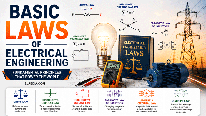
Ohm’s Law, Kirchhoff’s laws, Faraday’s Law, and Coulomb’s Law form the core basic electrical engineering laws used to analyze any electric circuit or electromagnetic system.
Each law in this guide is presented with the person behind it, the formal statement, standard equations, and real-world applications in electrical engineering.
Laws of electromagnetic induction – including Faraday’s Law, Lenz’s Law, Fleming’s hand rules, Biot–Savart Law, Ampère’s Circuital Law, and the Lorentz Force Law – are essential for designing machines, transformers, and power systems.
This article serves as a practical study guide for students and engineers preparing for exams, interviews, and field work.
A short FAQ at the end clarifies common doubts such as when Ohm’s Law fails, the difference between KCL and KVL, and whether these laws hold at high frequencies.

Introduction to Basic Electrical Engineering Laws

The fundamental laws of electrical engineering are called “fundamental” because they express conservation of charge, energy, and flux in any electric circuit or electromagnetic field. Without them, analyzing even basic electrical circuits would be guesswork.

These basic laws form the foundation for everything from simple DC networks to complex power grids and modern electronics. They originate from experimental work spanning roughly 1785 (Coulomb) through the early 20th century (Lorentz, Paschen).

Before diving in, here are the core quantities you’ll encounter throughout: voltage (V, in volts), electric current (I, in amperes), resistance (R, in ohms), charge (q, in coulombs), electric field (E, in V/m), magnetic field (B, in tesla), and power (P, in watts).

The laws covered fall into four categories: circuit laws (Ohm, Kirchhoff, Watt, Joule), field laws (Coulomb, Gauss, Biot–Savart, Ampère, Lorentz), induction laws (Faraday, Lenz, Fleming rules, Cork Screw Rule), and breakdown laws (Paschen).

These important laws are routinely applied in power systems, electronics, renewable energy, signal processing, and EV charging infrastructure.

Core Circuit Law: Ohm’s Law

Georg Simon Ohm, a German physicist, published Ohm’s Law in 1827 in his work Die galvanische Kette, mathematisch bearbeitet.

Ohm’s Law states that, “At constant temperature, the electric current through a conductor is directly proportional to the voltage across it and inversely proportional to its resistance“.

The standard equations are:

Form	Equation	Use
Voltage	V = I · R	Find voltage from current and resistance
Current	I = V / R	Find current from voltage and resistance
Resistance	R = V / I	Find resistance from voltage and current

One ohm is the resistance when one volt produces one amp. Ohm’s Law relates voltage, current, and resistance linearly and applies to both individual components and entire circuits.

When it applies and when it doesn’t:

Works for ohmic, linear circuits at constant temperature
Fails for diodes, transistors, thermistors, and gas-discharge lamps (non-linear devices)
In AC analysis, the relationship generalizes to V = I · Z, where Z is complex impedance – AC circuit principles extend Ohm’s Law to alternating current with complex impedance

Applications: It is used for sizing resistors in basic electrical circuits, calculating line current from supply voltage and load resistance, estimating voltage drops in cables, and troubleshooting by measuring V and I to infer a faulty R.

Power Relationships: Watt’s Law and Joule’s Law

Beyond current and voltage, electrical engineering needs power and energy laws to design safe, efficient electrical systems. Electrical power calculations are vital for determining component ratings and specifications.

Watt’s Law, associated with James Watt, gives the core equation P = V · I, with derived forms P = I^²R and P = V^²/R. Power P is measured in watts (W). For example, a 100 W lamp on 230 V mains draws approximately 0.43 A – a quick calculation using P = V · I.

Joule’s Law of heating, credited to James Prescott Joule (1840s), states the heat produced in a resistor is H = I^² · R · t, where H is electrical energy converted to heat in joules. This law explains the working principle behind the conversion of electrical energy into thermal energy.

Applications:

Design of electric heaters, kettles, and toasters
Fuse and circuit breaker sizing (ensuring elements open at correct current/time)
Thermal considerations in cable sizing and PCB trace width
Avoiding overheating in power electronics and inductor series connections

Kirchhoff’s Laws for Electric Circuits (KCL and KVL)

Gustav Kirchhoff, a German physicist, developed his laws in 1845 to extend Ohm’s Law to complex networks with many branches and loops. Kirchhoff’s laws are the backbone of circuit theory.

Kirchhoff’s current law expresses conservation of charge at a node, while Kirchhoff’s voltage law expresses conservation of energy around a closed loop. Both apply to DC and AC circuits and form the basis of nodal analysis and mesh analysis.

Kirchhoff’s Current Law (KCL)

Kirchhoff’s current law states that the algebraic sum of all the currents at any node equals zero. In plain terms, the total current entering a node equals the total current leaving it. KCL ensures charge conservation at electrical junctions – no charge can accumulate indefinitely at a point in a steady-state electric circuit.

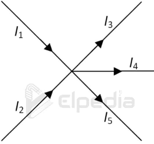
At the junction or node,

ΣI_entering = ΣI_leaving

I1 + I2 = I3 + I4 + I5

ΣI = 0 (with sign convention: currents entering positive, charge leaving negative, or vice versa)

For example, if 4 A and 9 A enters a node and three branches leave, carrying 6 A, 3 A and 4 A respectively, then 4 + 9 − 6 − 3 – 4 = 0. So, KCL is satisfied.

Applications: It is used for calculating branch currents in parallel loads, sizing busbars and distribution boards, validating current measurements in protection testing, and designing current divider circuits.

Kirchhoff’s Voltage Law (KVL)

Kirchhoff’s voltage law states the algebraic sum of all the voltage rises and voltage drops around any closed loop network is zero. The total voltage supplied by sources equals the sum consumed by loads in the same loop.

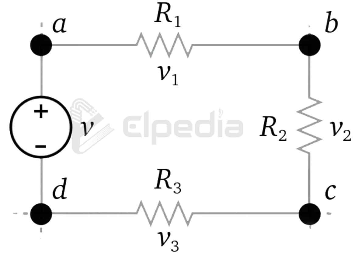
For a simple closed circuit with one voltage source and three resistors.

V − V₁ − V₂ − V₃ = 0

For example, if the supply voltage is 230 V, and voltage drop across the resistances R1, R2 and R3 are 80 V, 90 V and 60 V respectively. Then the total voltage in the closed path is given by, 230 – 80 – 90 – 60 = 0 V.

This rearranges to find unknown voltages or resistances. The voltage law KVL is essential for analyzing circuits with multiple voltage sources.

Applications: It is used for mesh analysis in multi-loop circuits, analyzing transformer equivalent circuits, studying voltage distribution in power system loops, and verifying correct wiring in panels.

Coulomb’s Law and the Basics of Electric Force

Charles-Augustin de Coulomb (French physicist, 1785) quantified the electrostatic force between two point charges using a torsion balance.

Coulomb’s Law describes the electrostatic force between two charges. It states that, “the force between two charges is directly proportional to the product of the charges and inversely proportional to the square of the distance between them”, acting along the straight line joining them. It is expressed as,

$F = \frac{k. \, (q_1 \, . \, q_2)}{r^2}$

Where q_₁ and q_₂ are in coulombs, r in meters, F in newtons, and k = 1/(4πε_₀) ≈ 8.988 × 10^⁹ N·m^²/C^². Like charges repel; unlike charges attract.

Applications: Coulomb’s law is used for estimating forces in high-voltage insulators and capacitors, understanding charge behavior on conductors, and forming the basis for electric field concepts used throughout electrostatic design.

Gauss’s Law and Electric Flux

Gauss’s Law, attributed to Carl Friedrich Gauss and formalized within Maxwell’s equations, relates the total electric flux through a closed surface to the enclosed charge. Its equation is written as,

$\iint_S E.dA = \frac{Q_{\text{enclosed}}}{\epsilon_0}$

In intuitive terms, electric flux counts the number of field lines crossing a surface. Symmetry – spherical, cylindrical, or planar – makes Gauss’s Law exceptionally powerful. For example, the electric field outside a uniformly charged sphere behaves identically to that of a point charge at the center, while inside the field depends on the enclosed charge only.

Applications: It is used for calculating fields in high-voltage equipment, analyzing charge distribution on conductors, designing coaxial cables and shielding, and forming part of Maxwell’s equations that underpin all electromagnetic theory.

Magnetic Fields and Current: Biot–Savart Law and Ampère’s Circuital Law

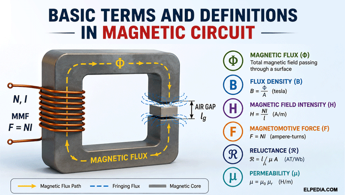
Electric current flowing through a conductor creates a magnetic field around it. The Biot–Savart Law and Ampère’s Circuital Law are fundamental laws used to calculate those fields. They are essential for understanding inductors, transformers, motors, and generators.

Biot–Savart Law

Credited to Jean-Baptiste Biot and Félix Savart (French scientists, early 1820s), the Biot–Savart Law gives the magnetic field contribution of a small current element, whose equation is given as,

$dB = \frac{\mu_0}{4\pi} \, \frac{I.dl \times \hat{r}}{r^2}$

The full field B is obtained by integrating over the entire current path. The magnitude and direction of the field depend on the geometry of the conductor.

Applications: It is used for estimating magnetic fields around busbars and transmission lines, designing inductors and electromagnets, and computing field strength in magnetic sensors.

Ampère’s Circuital Law

André-Marie Ampère (French physicist, 1820s) stated that the line integral of the magnetic field around a closed path equals μ_₀ times the total current enclosed, given by,

$\oint B.dl = \mu_0 I_{\text{enclosed}}$

For a long straight conductor: B = μ_₀I / (2πr). For a solenoid: B ≈ μ · n · I, where n is turns per meter.

Applications: It is used for magnetic circuit design in transformers and reactors, evaluating short-circuit forces in busbars, and analyzing current distribution in cables.

Electromagnetic Induction: Faraday’s Law, Lenz’s Law, Fleming’s Hand Rules, and Cork Screw Rule

Michael Faraday’s experiments in 1831 discovered electromagnetic induction, directly enabling electric generators and the modern power system. Understanding electromagnetic induction is key for deciphering the workings of motors and generators.

Faraday’s Law quantifies the induced electromotive force, Lenz’s Law determines its direction, and the hand rules provide quick visualization tools.

Faraday’s Law of Electromagnetic Induction

Faraday’s first law of electromagnetic induction states that “whenever the magnetic flux linking a closed circuit changes, an electromotive force is induced”.

Faraday’s second law of electromagnetic induction states that, “the induced EMF is proportional to the rate of change of flux”. The equation for Faraday’s Law is:

$E = - N \, \frac{d\phi}{dt}$

where N is the number of turns and Φ is the magnetic flux in webers. Faraday’s Law states induced EMF equals negative change in magnetic flux – the negative sign represents Lenz’s Law.

Faraday’s Law is fundamental for generators and transformers, and it is a cornerstone used in almost all energy conversion devices, from induction cooktops to wireless charging coils.

Lenz’s Law

Lenz’s Law is named after Heinrich Lenz, who established it in 1834. Lenz’s Law states that the induced current flows in a direction such that it opposes the change in magnetic flux that produced it. It is expressed as,

$E = - \frac{d\phi}{dt}$

The induced EMF’s direction is determined by Lenz’s Law, and Lenz’s Law is a consequence of the conservation of energy – mechanical work must be done to maintain flux changes.

Examples: dropping a magnet through a copper tube (braking effect), eddy-current braking in trains, and damping in analog meters.

Design applications: It is used for minimizing eddy-current losses in transformer cores through lamination, producing controlled braking in electromagnetic brakes, and designing speed sensors.

Flemings’ Right Hand rule

Attributed to John Ambrose Fleming (British engineer), the Right Hand Rule applies to generators. Fleming’s Right Hand rule states

Stretch out the fore finger, middle finger and thumb of your right hand in such a way that they are mutually perpendicular to each other. If the fore finger represents the direction of field(F), the thumb points in the direction of motion or applied force(B), then middle finger points in the direction of the induced current(I).

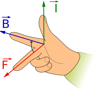
This rule lets you predict current direction in a rotating generator coil or in any conductor moving through a magnetic field.

Flemings’ Left Hand rule

Fleming’s left-hand Rule shows the direction of motion of motor. Fleming’s Left Hand rule states

Stretch out the fore finger, middle finger and thumb of your left hand in such a way that they are mutually perpendicular to each other. If the fore finger represents the direction of the field(B) and the middle finger represents that of the current(I), then thumb gives the direction of the force(F).

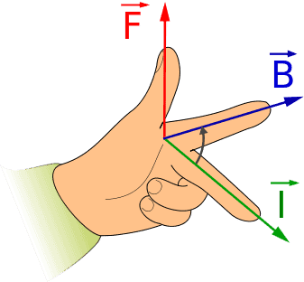
This rule is widely used to visualize motor operation, loudspeakers, and electromechanical actuators. It connects directly to the Lorentz force principle for predicting the direction of force on a current-carrying conductor.

Cork Screw Rule (Right-Hand Screw Rule)

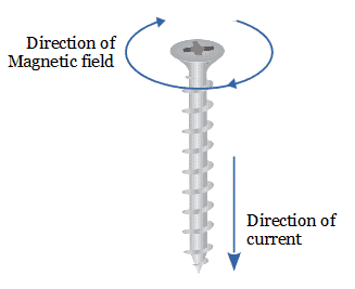
The Cork Screw Rule provides another way to determine the relationship between current and magnetic field. If a right-handed screw advances in the direction of current, the rotation shows the direction of magnetic field lines around the conductor.

It is often used alongside the Right Hand Rule to determine the polarity of electromagnets and predict induced magnetization in transformer windings.

Cork screw rule is one of the basic laws of electrical engineering

Lorentz Force Law and Motion of Charges in Fields

Hendrik Antoon Lorentz (Dutch physicist, late 19th century) described the force on a charged particle in combined electric and magnetic fields, expressed as,

F = q · (E + v × B)

Where q is charge in coulombs, v is velocity in m/s, and F is force in newtons. For current-carrying conductors, this becomes F = I · L × B, linking directly to Fleming’s Left Hand Rule.

Applications: It is used for calculating force on motor windings, designing Hall effect sensors, magnetic deflection in CRTs, and analyzing charged particle motion in mass spectrometers. The Lorentz Force Law is the underlying principle behind most electromechanical energy conversion devices.

Paschen’s Law and Electrical Breakdown

Friedrich Paschen (German physicist, 1889) studied breakdown voltages of gases between electrodes. Paschen’s Law states that the breakdown voltage V_b depends on the product of gas pressure (p) and gap distance (d).

V_b = f (p · d)

The Paschen curve for air shows a minimum breakdown voltage of approximately 327 V at a specific p·d value. At very small gaps or very large gaps, breakdown behavior changes significantly.

Applications: insulation coordination in high-voltage switchgear, design of gas-insulated substations, vacuum interrupters, and setting creepage and clearance distances in PCB design and safety standards.

Additional Important Laws and Concepts in Basic Electrical Engineering

Beyond the major laws, several supporting principles round out the basics of electrical engineering:

Conventional vs. electron current: conventional current flows from positive to negative; electrons move the opposite way. Pick one convention and stick with it.
ELI the ICE Man: in AC circuits, voltage leads current in an inductor (ELI) and current leads voltage in a capacitor (ICE) – a handy mnemonic for phase relationships.
Faraday’s Laws of Electrolysis (1833–1834): mass deposited at an electrode is proportional to total charge passed, with applications in plating and battery design.
Superposition Theorem: the response in any branch of a linear circuit equals the algebraic sum of responses from each independent source acting alone.
Maximum Power Transfer Theorem: maximum power is transferred when load resistance equals source resistance.
Thevenin’s and Norton’s Theorems: these allow simplification of complex electrical circuits into equivalent sources, making analysis of linear circuits far more manageable.

Maxwell’s equations describe how electric and magnetic fields interact and are fundamental to electromagnetism. In more advanced study, all the basic laws discussed here are unified under Maxwell’s framework, but for most power and circuit problems, the individual laws are sufficient.

Applications of Basic Laws in Modern Electrical Engineering

These basic laws of electrical engineering connect directly to every major subfield. Solar inverter designers use KCL, KVL, and Ohm’s Law daily to size components and verify circuit behavior.

Transformer engineers rely on Faraday’s Law, Ampère’s Law, and Lenz’s Law to optimize turns ratios, core materials, and loss characteristics. High-voltage transmission insulation is coordinated using Gauss’s Law and Paschen’s Law.

In protection systems, Watt’s and Joule’s Laws help engineers calculate fault currents and thermal effects on conductors. Data-center busway designs use KCL and Biot–Savart calculations to manage current sharing and magnetic effects.

Even with advanced simulation tools like SPICE and electromagnetic solvers, engineers still rely on these fundamental laws to cross-check results, interpret simulations, and make safe design decisions.

Students should practice deriving simple circuits and field problems from these laws to build strong intuition before relying on calculators or simulation software.

Frequently Asked Questions (FAQ)

Ohm’s Law assumes a linear, constant-temperature relationship between voltage and current. It fails for devices like diodes, transistors, thermistors, and gas-discharge lamps where the I–V curve is non-linear.

For such components, engineers use I–V characteristic curves from datasheets, piecewise-linear approximations, or SPICE models instead of a single constant resistance value.

KCL deals with currents at a node – it enforces conservation of charge so that the algebraic sum of currents entering and leaving equals zero. KVL deals with voltages around a closed loop – it enforces conservation of energy so that all voltage gains and losses sum to zero. KCL is the basis of nodal analysis, while KVL is the basis of mesh analysis. Both are valid in DC and AC circuits under normal lumped-element conditions.

At very high frequencies, parasitic inductances, capacitances, and finite signal propagation speed become significant. The lumped-circuit assumptions behind simple KCL and KVL break down, and full Maxwell’s equations or transmission line theory must be used. The underlying conservation principles remain the same, but the mathematical treatment changes to account for distributed effects, impedance matching, and reflection coefficients.

Faraday’s Law gives the magnitude of induced EMF in transformer windings (E = −N · dΦ/dt), while Lenz’s Law dictates the polarity so that resulting induced current flows to oppose the change in flux. In practice, this explains why primary current increases when a load is connected on the secondary – the secondary current creates an opposing flux, requiring more primary current to maintain core flux. Core design and lamination are critical to controlling this flux and minimizing losses.

Even though discrete charges are rarely manipulated directly in power or electronics circuits, Coulomb’s Law and Gauss’s Law define how charges and electric fields behave in and around conductors and insulators.

They are essential for designing capacitors, high-voltage insulation, electrostatic shielding (Faraday cages), and understanding phenomena like corona discharge and partial discharges in power equipment. Without these field laws, safe high-voltage design would be impossible.

Basic Laws of Electrical Engineering

Key Takeaways

Introduction to Basic Electrical Engineering Laws

Core Circuit Law: Ohm’s Law

Power Relationships: Watt’s Law and Joule’s Law