Mesh Analysis

Mesh analysis is a systematic circuit analysis technique used to determine unknown currents and voltages in electrical circuits.

It reduces the number of equations needed to analyze a circuit by assigning a current to each mesh and applying Kirchhoff’s Voltage Law (KVL) to the resulting loops.

At Elpedia, mesh analysis is presented as a fundamental circuit analysis method alongside nodal analysis. Mesh analysis is based primarily on Kirchhoff’s Voltage Law and Ohm’s law.

The method assigns a mesh current to each mesh—the smallest closed loop in a planar circuit—and uses these currents to determine the required branch currents and voltages.

Mesh analysis is applicable to planar circuits, which are circuits that can be drawn on a two-dimensional surface without branches crossing each other except at actual nodes. For non-planar circuits, nodal analysis is generally a more suitable alternative.

This article explains the concepts of loops, meshes, and mesh currents, the relationship between mesh analysis and Kirchhoff’s Voltage Law, the step-by-step procedure for solving circuits, and special cases such as supermesh analysis and circuits with dependent sources. Several worked examples are also included to demonstrate how mesh analysis is applied to practical electrical circuits.

What is Mesh Analysis?

Mesh analysis, also known as the mesh current method, is a systematic circuit analysis technique used to determine unknown currents and voltages in a planar circuit.

The method assigns a mesh current to each mesh and applies Kirchhoff’s Voltage Law (KVL) to obtain a set of simultaneous equations.

A mesh is the smallest closed loop in a planar circuit that does not contain another loop within it.

In mesh analysis, a current is assigned to each mesh, usually in the same direction, such as clockwise. These assigned currents are called mesh currents.

Mesh currents are assumed circuit variables and do not always correspond directly to physical branch currents. If a circuit element belongs to only one mesh, its branch current is equal to the corresponding mesh current.

If an element is shared by two meshes, its branch current is the algebraic difference of the two mesh currents. For example, if $I_1$ and $I_2$ flow through a shared resistor in opposite directions,

The direction chosen for the mesh currents is arbitrary, but it must be used consistently when writing the KVL equations.

For a planar circuit with $n$ independent meshes, mesh analysis produces $n$ independent equations in the $n$ mesh currents. Solving these equations gives the mesh currents, from which the required branch currents and voltages can be determined.

Mesh analysis can also be extended to AC circuits by replacing resistance with complex impedance and expressing voltages and currents as phasors. In this article, the basic worked examples primarily consider DC resistive circuits.

Why Mesh Analysis is Used in Circuit Analysis

Mesh analysis provides a systematic way to analyze electrical circuits by reducing the number of unknown variables and equations required.

Instead of determining the current in every branch independently, the method assigns one current to each mesh and uses Kirchhoff’s Voltage Law (KVL) to develop equations for those mesh currents.

For a planar circuit with a relatively small number of meshes, this approach can produce a compact set of simultaneous equations.

Once the mesh currents are determined, the currents and voltages in individual branches can be calculated from them. This makes mesh analysis particularly useful for circuits containing multiple voltage sources and series-connected resistive elements.

Mesh analysis is one of the two major systematic methods of circuit analysis, along with nodal analysis. Mesh analysis is based primarily on KVL and is often convenient when a circuit has fewer meshes than independent node-voltage variables.

Nodal analysis, which is based on Kirchhoff’s Current Law (KCL), may be more convenient for circuits with many current sources or fewer essential nodes.

Another advantage of mesh analysis is its systematic procedure: assign mesh currents, apply KVL to each mesh, form the equations, and solve for the unknown currents. The method also helps illustrate the relationship between voltage drops, circuit currents, and the conservation of energy represented by KVL.

Therefore, mesh analysis is particularly useful when the circuit is planar and contains a relatively small number of meshes, allowing the circuit to be analyzed with a manageable number of equations.

Relationship Between Mesh Analysis and Kirchhoff’s Voltage Law (KVL)

Kirchhoff’s Voltage Law (KVL) is the fundamental principle used in mesh analysis. KVL states that the algebraic sum of all voltage rises and voltage drops around any closed loop is zero. Since each mesh is a closed loop, a KVL equation can be written for every mesh.

When writing a mesh equation, you traverse the mesh in the chosen direction of the assigned mesh current and account for each voltage rise and voltage drop encountered. For example, a simple mesh equation may be written as

The sign of each term depends on the chosen direction of the mesh current and the polarity of the voltage sources in the circuit.

When a resistor is shared by two meshes, the current through that resistor is determined by the algebraic difference between the corresponding mesh currents.

For example, if resistor R₃ is common to mesh 1 and mesh 2, and I₁ and I₂ flow through the resistor in opposite reference directions, then the voltage drop across the shared resistor is

While KVL is used explicitly in mesh analysis, Kirchhoff’s current law appears implicitly at shared branches and explicitly when forming supermeshes around current sources.

When is Mesh Analysis Especially Useful?

Mesh analysis is particularly useful for planar circuits that have a relatively small number of meshes. The method can be especially convenient when:

• The circuit has fewer meshes than independent node-voltage variables.
• The circuit contains several voltage sources, which can be incorporated directly into the KVL equations.
• The circuit contains resistors and other elements arranged within well-defined meshes.
• The required quantities are branch currents or mesh currents.

For example, consider a planar circuit containing three independent meshes. Mesh analysis requires three mesh-current equations, one for each mesh.

Depending on the circuit topology, nodal analysis may require a different number of node-voltage equations.

Therefore, the more appropriate method depends on the number of independent unknowns and the type of sources present, rather than simply on the number of branches.

Mesh analysis can also be used in circuits containing current sources. If a current source belongs to only one mesh, it directly determines that mesh current.

If a current source lies between two meshes, a supermesh and an additional current constraint are used.

In general, mesh analysis is a convenient choice for planar circuits with a relatively small number of meshes, particularly when voltage sources are prominent.

For circuits with many current sources or many nodes but relatively few essential nodes, nodal analysis may provide a more convenient formulation.

What is a Mesh, a Loop, and an Essential Mesh?

Understanding the difference between a loop and a mesh is important before applying mesh analysis.

A loop is a closed path in an electrical circuit that does not pass through the same node more than once, except for the starting node. A circuit can contain several different loops, including both small loops and larger loops that enclose other loops.

A mesh is a loop that does not contain any other loop within it. In a planar circuit, meshes correspond to the smallest closed regions of the circuit diagram. These are the loops used in the mesh-current method.

For example, consider a rectangular circuit divided into two sections by a central resistor. The outer boundary forms a loop, but it is not a mesh because it contains two smaller loops. Each of the two smaller sections is a mesh because neither contains another loop within it.

An essential mesh is an independent mesh used to formulate the mesh-current equations of a planar circuit. One mesh current is assigned to each independent mesh, and one independent KVL equation is written for each mesh.

For a connected planar circuit, the number of independent meshes is m = b – n + 1 where m = number of independent meshes, b = number of branches and n = number of nodes.

This relationship gives the number of independent mesh equations required for mesh analysis.

The direction of each mesh current is arbitrary. However, choosing the same direction for all mesh currents, usually clockwise, can make the KVL equations easier to formulate and reduce sign errors.

Basic Principle Behind Mesh Analysis

The basic idea of mesh analysis is to replace the unknown branch currents in a planar circuit with a smaller set of mesh currents.

A mesh current is assigned to each mesh, and Kirchhoff’s Voltage Law (KVL) is then applied to each mesh to obtain a set of simultaneous equations.

Once the mesh currents are determined, the actual currents in individual branches can be calculated from them.

The relationship between mesh currents and branch currents depends on how a branch is connected:

• Branch belonging to one mesh: The branch current is equal to the corresponding mesh current.
• Branch shared by two meshes: The branch current is the algebraic difference between the two mesh currents.

Ohm’s law is used to express the voltage across a resistive element in terms of its current. KVL is then used to relate the voltage drops and voltage sources around each mesh. Combining these relationships produces the mesh-current equations.

Steps to solve mesh analysis method

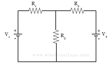
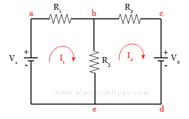
Consider a simple circuit as shown in the below figure.

1. Make sure that the circuit considered for analysis has only voltage sources. If there is any current source in the circuit, use the source transformation method and convert it into a voltage source.
2. Label the nodes with either numbers or alphabets.
3. Assign the mesh currents in each loop, such that all the current directions are in a clockwise direction.

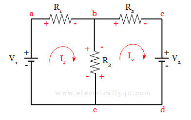
4. Along the assumed direction of the current, mark the polarities of a voltage drop across each element. While doing, assign the correct polarity of the voltage source.

5. For each loop, write the current equation by applying KVL to each loop.
6. If two currents are flowing in the same branch, it is called a shared branch. In this circuit, mesh currents I₁ and I₂ are flowing through R₃(Branch ‘be‘).
7. Now, just look at the circuit. For loop1[abea], the current direction is assumed to be from ‘b to e‘, the current will be I₁ – I₂. But for loop2[bcdeb], the current direction is assumed to be from ‘e to b‘, so the current will be I₂ – I₁.

For the above circuit, apply KVL to loop1 and loop2 to get two equations

8. The above two equations are solved by using Cramer’s rule, to obtain the solutions.
9. If the obtained solution is negative, then the actual direction of the current is opposite to that of the assumed direction.

Assigning Mesh Currents and Sign Conventions

The way mesh currents are assigned and voltage polarities are handled affects the clarity of the KVL equations and helps reduce algebraic errors.

Assign a mesh current to each mesh. The direction of each mesh current is arbitrary, but assigning all mesh currents in the same direction—usually clockwise—is a common and convenient convention. Consistent current directions make it easier to formulate the KVL equations for adjacent meshes.

For a resistor shared by two meshes, the branch current is the algebraic difference between the two mesh currents. For example, if $I_1$ and $I_2$ are clockwise mesh currents, the current through a shared resistor $R$, referenced in the direction of $I_1$, is:

Therefore, the voltage drop across the resistor in the direction of $I_1$ is:

When writing the KVL equation for mesh 2, the same resistor is traversed in the opposite reference direction, giving:

The sign of a voltage source in a KVL equation depends on the direction in which the source is traversed:

• Traversing from the negative terminal to the positive terminal (in the direction of the mesh current) counts as a voltage rise (+V).
• Traversing from positive to negative counts as a voltage drop (−V).

The source polarity and the chosen mesh-current direction must therefore be considered when writing each KVL equation.

A negative value for a calculated mesh current does not indicate an error. It means that the actual current flows in the direction opposite to the direction initially assumed.

For example, if the calculated value is I₂ = -1.5 A, the actual mesh current is $1.5\text{ A}$ in the direction opposite to the assumed direction of I₂.

Handling Current Sources and Supermesh in Mesh Analysis

Current sources require special treatment in mesh analysis because their current is known, but their voltage is generally unknown. Therefore, a conventional KVL equation cannot be written directly across an ideal current source because its voltage is not known.

If an independent current source is present only in one mesh, the current source directly determines that mesh current. Thus, I_mesh = ± Is.

The sign depends on whether the direction of the current source is the same as or opposite to the assumed mesh-current direction. In this case, a separate KVL equation is not required for that mesh.

A supermesh is formed when a current source lies on the common branch between two adjacent meshes.

Since the voltage across the current source is unknown, a KVL equation cannot be written directly around either mesh. Instead, the two meshes are combined to form a larger loop called a supermesh.

To analyze a supermesh:

1. Identify the current source shared by the two meshes.
2. Combine the two adjacent meshes into a supermesh.
3. Write a KVL equation around the outer boundary of the supermesh, excluding the branch containing the current source.
4. Write an additional current-source constraint relating the two mesh currents.
5. Solve the resulting simultaneous equations.

A dependent current source located on a common branch between two meshes is handled using the same supermesh concept. The additional constraint is determined by the value of the dependent source and its controlling variable.

Solved Problem 1

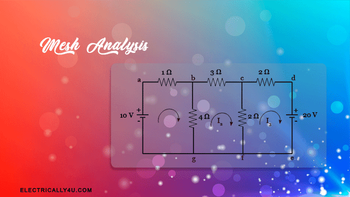
Determine the mesh currents in the circuit shown below.

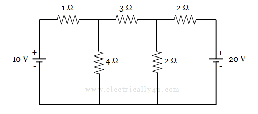
The given circuit is redrawn by assigning the current and its direction in each loop and the nodes are labelled.

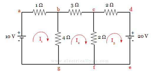
Along the direction of the current, the polarities of voltage drop are marked for each element. The circuit is redrawn with polarities as drawn below.

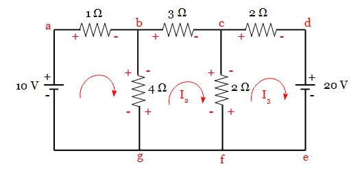
Now, from the above circuit diagram, we can observe that, there are three loops(Loop1: abga, Loop2: bcfgb, Loop3: cdefc). Each loop carries a current I₁, I₂ and I₃ respectively.

Apply KVL to loop1[abga], we get,

Apply KVL to loop2[bcfgb],

Apply KVL to loop3[cdefc],

The above three equations are written in matrix form, as shown below,

Applying Cramer’s rule, we get

Now, the value of current in each loop is determined

The loop currents I₂ and I₃ have negative values, which means the actual current direction is opposite to the assumed direction.

Current through the branch ‘bg’ is I₁ – I₂ = 1.664 + 0.416 = 2.08 A

Current through the branch ‘cf’ is I₂ – I₃ = -0.416 + 5.21 = 4.794 A

Solved Problem 2

For the circuit shown below, determine the mesh currents and branch currents using mesh analysis.

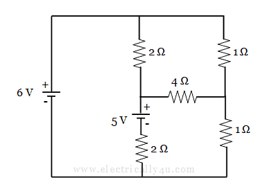
For the given circuit, let us label the nodes and assign the mesh currents. The circuit is redrawn as shown below. The polarities are also marked across each element in the circuit.

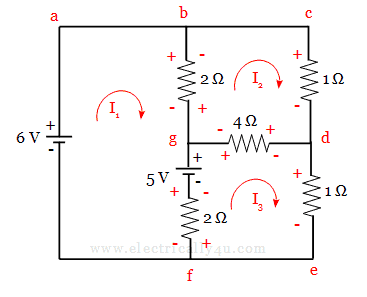
In this circuit, you can observe that, there are three loops and each loop carries current I₁, I₂ and I₃. To determine the current values, let us apply Kirchoff’s voltage Law to each loops.

Apply KVL to loop1[abgfa], we get,

Apply KVL to loop2[bcdgb],

Apply KVL to loop3[gdefg],

The above three equations are written in matrix form, as shown below,

Applying Cramer’s rule, we get

Now, the value of current in each loop is determined as follows

The branch currents are determined as follows

In branch bg, I_bg = I₁ – I₂ = 3.25 – 2.77 = 0.48 A

In branch fg, I_fg = I₃ – I₁ = 3.23 – 3.25 = -0.02 A

In branch gd, I_gd = I₃ – I₂ = 3.23 – 2.77 = 0.46 A

Solved Problem 3

For the circuit shown below, determine the mesh currents and branch currents using mesh analysis.

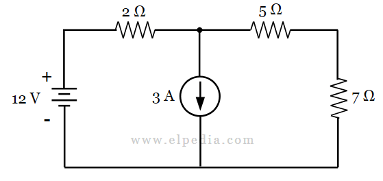
For the given circuit, let us label the nodes and assign the mesh currents. The circuit is redrawn as shown below. The polarities are also marked across each element in the circuit.

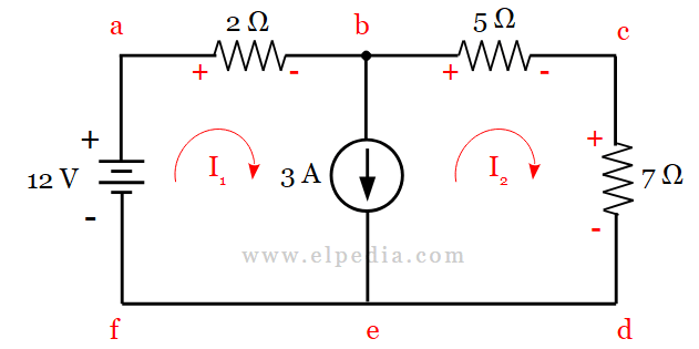
Since the 3 A current source is in the common branch, we cannot write an ordinary KVL equation for each mesh separately. We use the current-source constraint + a supermesh KVL equation.

In the shared branch, $I_1$ flows downward and $I_2$ flows upward. Therefore,

Since the current-source branch is excluded, go around the outer loop containing the 12 V source, 2 Ω, 5 Ω, and 7 Ω.

Applying KVL for this outer supermesh [abcdefa],

Sub eqn.(1) in the above equation,

Now, from equation (1),